
PCGCv2
PCGCv2, Multiscale, point cloud compression, deeplearning
PCGCv2, is a kind of point cloud lossy compression method, and the source code uses pytorch as deeplearning framework.
Paper citation:
@INPROCEEDINGS{9418789, author={Wang, Jianqiang and Ding, Dandan and Li, Zhu and Ma, Zhan}, booktitle={2021 Data Compression Conference (DCC)}, title={Multiscale Point Cloud Geometry Compression}, year={2021}, volume={}, number={}, pages={73-82}, doi={10.1109/DCC50243.2021.00015}}
our contributions
1.benchmark test on different PC files, and on different metrics, including bpp, D1, D2, time, compared with PCGCv1.
2.draw a flow chart about encoding process.
3.BD-BR and BD-PSNR calculation over GPCC(octree), also compared with PCGCv1.
file structure
root
└── mpeg-pcc-tmc13-master: gpcc compression software
└── PCGCv2-master: source code
└── Multiscale Point Cloud Geometry Compression.pdf: origional paper
└── PCGCv2 explanation.docx: introduction for paper, performance, instructions
└── flowchart.vsdx: flow chart about encoding process
└── dataset: training_dataset.zip, test data
environment
- ubuntu 18.04
- cuda V10.2.89
- python 3.6.9
- MinkowskiEngine 0.5 or higher (for sparse convolution) We recommend you to follow https://github.com/NVIDIA/MinkowskiEngine to setup the environment for sparse convolution.
- refer to requirements-pytorch.txt
command
cd PCGCv2-master
chmod +x tmc3
chmod +x pc_error_d
encode and decode:
python coder.py --filedir="/userhome/PCGCv1/pytorch_eval/28_airplane_0270.ply" --ckptdir='ckpts/r7_0.4bpp.pth'
You can get some test files here
Training:
python train.py --dataset='../../training_dataset/' --init_ckpt='ckpts/r3_0.10bpp.pth' --epoch=300
performance
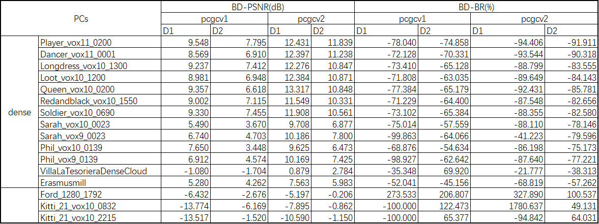
We first caculate the BD-PSNR and BD-BR rate of PCGCv2, PCGCv1 over GPCC(octree), the result shows as below. We can see from the table, that for dense PCs, PCGCv2 gets better performance than octree, while for sparse PCs, it gets worse. It is almost the same for PCGCv1, except for VillaLaTesorieraDenseCloud. The main reason is that there is no sparse PC data in training sets, so the model can not learn the features. And compared with PCGCv1, PCGCv2 is better, no matter for dense or sparse PCs.
We then carry out a benchmark test on PC files including those are not tested by author. The part of the result shows as below, others please go to /results. From the result, we can see that PCGCv2 gets better performance in bpp, d1, d2, as well as time. It seems to be a perfect solution for lossy PCC. But in practice, we found that PCGCv2 uses too much GPU memory while coding, so it cannot be used for big PC files or in Edge Calculating Machines. And the reason is that PCGCv2 compresses the complete PC at the same time, while generally other methods would depart the PC into many small boxes and compress the boxes one by one.
| PCs |
resolution |
D2 PSNR(PCGCv2) |
D1 PSNR(PCGCv2) |
bpp(PCGCv2) |
time(enc)(PCGCv2) |
time(dec)(PCGCv2) |
D2 PSNR(PCGCv1) |
D1 PSNR(PCGCv1) |
time_enc(PCGCv1) |
time_dec(PCGCv1) |
bpp(PCGCv1) |
| basketball_player_vox11_00000200 |
2048 |
72.5485 |
70.0165 |
0.02 |
2.011 |
23.229 |
64.8938 |
55.0611 |
267.909 |
139.188 |
0.0756 |
| basketball_player_vox11_00000200 |
2048 |
78.7591 |
75.802 |
0.042 |
1.456 |
23.606 |
79.158 |
75.5727 |
211.993 |
95.08 |
0.1435 |
| basketball_player_vox11_00000200 |
2048 |
80.9193 |
77.8298 |
0.077 |
1.5 |
23.094 |
81.2816 |
78.2683 |
239.743 |
107.646 |
0.2023 |
| basketball_player_vox11_00000200 |
2048 |
83.0218 |
79.5694 |
0.133 |
1.383 |
23.67 |
82.8921 |
79.4893 |
238.08 |
104.54 |
0.2459 |
| basketball_player_vox11_00000200 |
2048 |
84.9523 |
81.1622 |
0.22 |
1.348 |
23.223 |
84.2958 |
80.5892 |
235.813 |
103.308 |
0.2944 |
| basketball_player_vox11_00000200 |
2048 |
85.8507 |
81.9518 |
0.29 |
1.664 |
23.892 |
85.5959 |
81.7542 |
232.871 |
97.416 |
0.3504 |
| basketball_player_vox11_00000200 |
2048 |
86.7934 |
82.7566 |
0.375 |
1.492 |
23.505 |
86.6172 |
82.611 |
236.226 |
114.151 |
0.4368 |
| phil_vox10_0139 |
1024 |
65.4011 |
62.8073 |
0.019 |
1.098 |
11.351 |
65.3935 |
59.2323 |
138.337 |
65.703 |
0.0819 |
| phil_vox10_0139 |
1024 |
69.4115 |
66.1906 |
0.038 |
1.127 |
12.658 |
70.1038 |
67.1497 |
97.99 |
46.637 |
0.1292 |
| phil_vox10_0139 |
1024 |
71.7819 |
68.9794 |
0.082 |
1.225 |
11.072 |
72.4775 |
69.0606 |
103.552 |
71.094 |
0.2078 |
| phil_vox10_0139 |
1024 |
73.5822 |
70.4359 |
0.139 |
1.136 |
11.374 |
73.7427 |
70.0563 |
94.865 |
46.052 |
0.2566 |
| phil_vox10_0139 |
1024 |
75.0323 |
71.5706 |
0.229 |
1.089 |
11.213 |
74.3338 |
70.3875 |
97.979 |
47.382 |
0.3121 |
| phil_vox10_0139 |
1024 |
75.4909 |
71.933 |
0.285 |
1.152 |
11.446 |
74.8807 |
70.9274 |
105.117 |
48.889 |
0.3787 |
| phil_vox10_0139 |
1024 |
75.9504 |
72.2833 |
0.351 |
1.193 |
11.002 |
75.1343 |
70.8476 |
109.787 |
54.19 |
0.4618 |
| sarah_vox9_0023 |
512 |
60.0831 |
57.1343 |
0.028 |
0.682 |
2.338 |
57.7055 |
50.695 |
33.071 |
17.38 |
0.0889 |
| sarah_vox9_0023 |
512 |
64.0241 |
60.6775 |
0.049 |
0.75 |
2.403 |
64.4054 |
61.5184 |
26.308 |
12.194 |
0.1417 |
| sarah_vox9_0023 |
512 |
66.3538 |
63.4667 |
0.093 |
0.436 |
2.501 |
67.2605 |
63.8802 |
27.383 |
12.014 |
0.2254 |
| sarah_vox9_0023 |
512 |
68.3318 |
64.9725 |
0.152 |
0.677 |
2.662 |
68.5138 |
65.0884 |
36.251 |
16.083 |
0.2746 |
| sarah_vox9_0023 |
512 |
69.9245 |
66.3328 |
0.247 |
0.805 |
2.406 |
69.2561 |
65.7159 |
34.676 |
12.428 |
0.3361 |
| sarah_vox9_0023 |
512 |
70.4951 |
66.6033 |
0.31 |
1.59 |
3.33 |
69.9792 |
66.3444 |
32.836 |
12.619 |
0.4053 |
| sarah_vox9_0023 |
512 |
71.001 |
66.961 |
0.384 |
0.815 |
2.494 |
70.3887 |
66.4396 |
32.061 |
15.015 |
0.5022 |
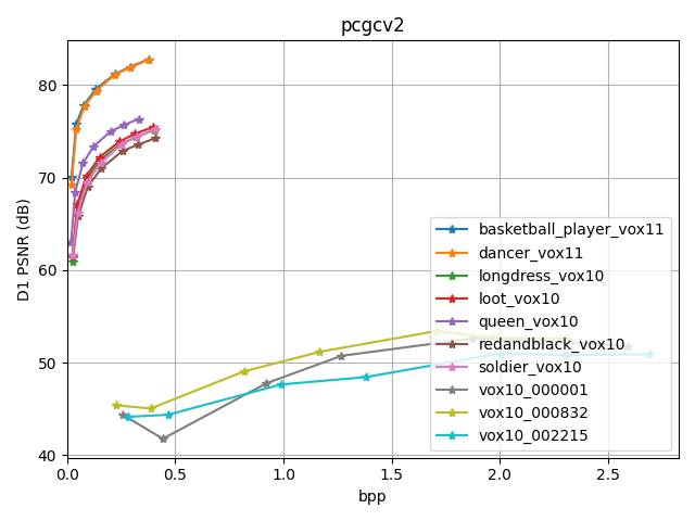
According to the results above, we draw D1-bpp and D2-bpp figures, to clearly show the performance between different PC files as below. It is obvious that, PCs of vox11 have best performance, which are on up-left part of the figure, PCs of vox10 are second in the middle, and PCs of sparse have bad performance on the bottom part.

Cite from:
https://github.com/NJUVISION/PCGCv2
The source code files are provided by Nanjing University Vision Lab. And thanks for the help from Prof. Dandan Ding from Hangzhou Normal University and Prof. Zhu Li from University of Missouri at Kansas. Please contact us (mazhan@nju.edu.cn and wangjq@smail.nju.edu.cn) if you have any questions.
contributors
name: Ye Hua
email: yeh@pcl.ac.cn